This website uses cookies to ensure you get the best experience on our website.
- Table of Contents

ELISA data is typically graphed with optical density vs log concentration to produce a sigmoidal curve. Known concentrations of antigen are used to produce a standard curve and then this data is used to measure the concentration of unknown samples by comparison to the linear portion of the standard curve. The relatively long linear region of the curve makes the ELISA results accurate and reproducible.
The unknown concentration can be determined directly on the graph or with curve-fitting software which is typically found on an ELISA plate reader. We will now solve your problems in the following article in the order of a typical experiment sequence.
In ELISA experiments, the general steps for calculating the standard curve are as follows:
Here is what we recommend (Best performed within 2 hours):
Note: When diluting the standard solution in a gradient, brief centrifugation after dilution is acceptable to allow any liquid adhering to the tube cap and wall to settle at the bottom, facilitating dilution for the next concentration. Using 200 µL per tube as an example, the dilution method is illustrated in the diagram below, and the dilution volume can be adjusted according to actual requirements.
We recommend drawing it using curve-fitting software and tools like CurveExpert, and GraphPad Prism. Microsoft Excel. Put all the data you measured in it, plotting the mean absorbance (y-axis) against the protein concentration (x-axis) and choosing the best-fit curve for the data points.
You can check ELISA Data Analysis Instructions for further information.
Put all the data you measured in it, plotting the mean absorbanceCurve fitting software will provide different model options for data plotting, including linear plots, semi-log plots, log/log plots, and 4- or 5-parameter logistic (4PL or 5PL) curves.
The simplest method is to use linear regression to fit the standard curve. After passing a linearity test, the formula for the standard curve is a simple linear equation: y=mx+b, where y is the signal intensity, x is the concentration, m is the slope, and b is the intercept. Semi-log or log/log scale can also be used when there is a large difference between the upper and lower limits of the determined concentration.
The five-parameter logistic fitting is a commonly used curve fitting method, while it is more complex and asymmetrical. If the data points suggest asymmetry near the plateaus, the 5PL curve would be useful. However, more data points must be collected to determine whether asymmetry exists. As a result, it is generally recommended to use the simpler 4-PL for the best standard curve fit.
The formula for the 4PL standard curve is typically represented as:
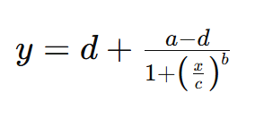
Where:
(In ELISA experiments, EC50 stands for Half Maximal Effective Concentration, which is commonly used to measure the affinity of antibodies to specific molecules. The EC50 value refers to the concentration at which the antibody achieves half of its maximum effect within a certain concentration range.)
The Limit of Detection (LoD) at which a target analyte can be reliably detected in a sample, but may not provide an accurate concentration value. The Limit of Quantification (LoQ) is the lowest concentration that can be accurately measured. At this concentration, the instrument can provide a reliable concentration value, and the precision and accuracy are within an acceptable range.
In theory, the "0" concentration point serves as both the lowest concentration point and the "detection limit". But as the huge impact the background noise affects and as the Lambert-Beer law fails at low concentrations, we usually set the LoD at three times bigger than the background noise. The LOQ needs to be adjusted by the experimenter according to the precision of the ELISA kit used in the experiment, and it should be greater than the LoD. We usually set LoQ at ten times bigger than the background noise.
Yes, Boster offers an Online ELISA Kit Calculator.
Put your result into the online calculator and select the output parameters. Wait a few minutes and you can download a PDF file or a CSV file containing the standard curve and analyzed data.
Linearity tests are usually used to examine the precision of the standard curve.
For a standard curve plotted from measurements obtained at 4 to 6 concentration units, spectrophotometric methods generally require the correlation coefficient |r| to be ≥0.9990. Otherwise, the reasons should be identified and corrected, and a qualified standard curve should be redrawn.
No one can guarantee assay accuracy once the concentrations outside the specified range within the curve are used. A specific range is generated to provide statistical confidence for the assay accuracy. Samples with absorbance values falling outside the range of the standard curve should be diluted before proceeding with ELISA staining for accurate results. When analyzing such samples, the concentration obtained from the standard curve should be multiplied by the dilution factor.
Many factors can influence the high standard OD value. The signal can vary according to the operator technique for the standard curve preparation, washing method, incubation variability, and plate reader calibration. The maximum assay signal is expected to measure between 1.0 and 3.5 OD.
The standard curve range has been validated for reliable and accurate performance across multiple kit lots and operators. The lowest standard concentration is the lowest limit that ELISA systems can guarantee for reliable assay measurements. Sample values extrapolated below the lowest standard concentration may not be accurate.